Abstract
Lots of learning tasks require dealing with graph data which contains rich relation information among elements. Modeling physics systems, learning molecular fingerprints, predicting protein interface, and classifying diseases demand a model to learn from graph inputs. In other domains such as learning from non-structural data like texts and images, reasoning on extracted structures (like the dependency trees of sentences and the scene graphs of images) is an important research topic which also needs graph reasoning models. Graph neural networks (GNNs) are neural models that capture the dependence of graphs via message passing between the nodes of graphs. In recent years, variants of GNNs such as graph convolutional network (GCN), graph attention network (GAT), graph recurrent network (GRN) have demonstrated ground-breaking performances on many deep learning tasks. In this survey, we propose a general design pipeline for GNN models and discuss the variants of each component, systematically categorize the applications, and propose four open problems for future research.
1. Introduction
Graphs are a kind of data structure which models a set of objects (nodes) and their relationships (edges). Recently, researches on analyzing graphs with machine learning have been receiving more and more attention because of the great expressive power of graphs, i.e. graphs can be used as denotation of a large number of systems across various areas including social science (social networks (Wu et al., 2020), natural science (physical systems (Sanchez et al., 2018; Battaglia et al., 2016) and protein-protein interaction networks (Fout et al., 2017)), knowledge graphs (Hamaguchi et al., 2017) and many other research areas (Khalil et al., 2017). As a unique non-Euclidean data structure for machine learning, graph analysis focuses on tasks such as node classification, link prediction, and clustering. Graph neural networks (GNNs) are deep learning based methods that operate on graph domain. Due to its convincing performance, GNN has become a widely applied graph analysis method recently. In the following paragraphs, we will illustrate the fundamental motivations of graph neural networks.
The first motivation of GNNs roots in the long-standing history of neural networks for graphs. In the nineties, Recursive Neural Networks are first utilized on directed acyclic graphs (Sperduti and Starita, 1997; Frasconi et al., 1998). Afterwards, Recurrent Neural Networks and Feedforward Neural Networks are introduced into this literature respectively in (Scarselli et al., 2009) and (Micheli, 2009) to tackle cycles. Although being successful, the universal idea behind these methods is building state transition systems on graphs and iterate until convergence, which constrained the extendability and representation ability. Recent advancement of deep neural networks, especially convolutional neural networks (CNNs) (LeCun et al., 1998) result in the rediscovery of GNNs. CNNs have the ability to extract multi-scale localized spatial features and compose them to construct highly expressive representations, which led to breakthroughs in almost all machine learning areas and started the new era of deep learning (LeCun et al., 2015). The keys of CNNs are local connection, shared weights and the use of multiple layers (LeCun et al., 2015). These are also of great importance in solving problems on graphs. However, CNNs can only operate on regular Euclidean data like images (2D grids) and texts (1D sequences) while these data structures can be regarded as instances of graphs. Therefore, it is straightforward to generalize CNNs on graphs. As shown in Fig. 1, it is hard to define localized convolutional filters and pooling operators, which hinders the transformation of CNN from Euclidean domain to non-Euclidean domain. Extending deep neural models to non-Euclidean domains, which is generally referred to as geometric deep learning, has been an emerging research area (Bronstein et al., 2017). Under this umbrella term, deep learning on graphs receives enormous attention.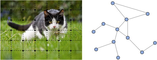
The other motivation comes from graph representation learning (Cui et al., 2018a; Hamilton et al., 2017b; Zhang et al., 2018a; Cai et al., 2018; Goyal and Ferrara, 2018), which learns to represent graph nodes, edges or subgraphs by low-dimensional vectors. In the field of graph analysis, traditional machine learning approaches usually rely on hand engineered features and are limited by its inflexibility and high cost. Following the idea of representation learning and the success of word embedding (Mikolov et al., 2013), DeepWalk (Perozzi et al., 2014), regarded as the first graph embedding method based on representation learning, applies SkipGram model (Mikolov et al., 2013) on the generated random walks. Similar approaches such as node2vec (Grover and Leskovec, 2016), LINE (Tang et al., 2015) and TADW (Yang et al., 2015) also achieved breakthroughs. However, these methods suffer from two severe drawbacks (Hamilton et al., 2017b). First, no parameters are shared between nodes in the encoder, which leads to computationally inefficiency, since it means the number of parameters grows linearly with the number of nodes. Second, the direct embedding methods lack the ability of generalization, which means they cannot deal with dynamic graphs or generalize to new graphs.
Based on CNNs and graph embedding, variants of graph neural networks (GNNs) are proposed to collectively aggregate information from graph structure. Thus they can model input and/or output consisting of elements and their dependency.
There exists several comprehensive reviews on graph neural networks. Bronstein et al. (2017) provide a thorough review of geometric deep learning, which presents its problems, difficulties, solutions, applications and future directions. Zhang et al. (2019a) propose another comprehensive overview of graph convolutional networks. However, they mainly focus on convolution operators defined on graphs while we investigate other computation modules in GNNs such as skip connections and pooling operators.
Papers by Zhang et al. (2018b), Wu et al. (2019a), Chami et al. (2020) are the most up-to-date survey papers on GNNs and they mainly focus on models of GNN. Wu et al. (2019a) categorize GNNs into four groups: recurrent graph neural networks, convolutional graph neural networks, graph autoencoders, and spatial-temporal graph neural networks. Zhang et al. (2018b) give a systematic overview of different graph deep learning methods and Chami et al. (2020) propose a Graph Encoder Decoder Model to unify network embedding and graph neural network models. Our paper provides a different taxonomy with them and we mainly focus on classic GNN models. Besides, we summarize variants of GNNs for different graph types and also provide a detailed summary of GNNs’ applications in different domains.
There have also been several surveys focusing on some specific graph learning fields. Sun et al. (2018) and Chen et al. (2020a) give detailed overviews for adversarial learning methods on graphs, including graph data attack and defense. Lee et al. (2018a) provide a review over graph attention models. The paper proposed by Yang et al. (2020) focuses on heterogeneous graph representation learning, where nodes or edges are of multiple types. Huang et al. (2020) review over existing GNN models for dynamic graphs. Peng et al. (2020) summarize graph embeddings methods for combinatorial optimization. We conclude GNNs for heterogeneous graphs, dynamic graphs and combinatorial optimization in Section 4.2, Section 4.3, and Section 8.1.6 respectively.
In this paper, we provide a thorough review of different graph neural network models as well as a systematic taxonomy of the applications. To summarize, our contributions are:
- •
We provide a detailed review over existing graph neural network models. We present a general design pipeline and discuss the variants of each module. We also introduce researches on theoretical and empirical analyses of GNN models.
- •
We systematically categorize the applications and divide the applications into structural scenarios and non-structural scenarios. We present several major applications and their corresponding methods for each scenario.
- •
We propose four open problems for future research. We provide a thorough analysis of each problem and propose future research directions.
The rest of this survey is organized as follows. In Section 2, we present a general GNN design pipeline. Following the pipeline, we discuss each step in detail to review GNN model variants. The details are included in Section 3 to Section 6. In Section 7, we revisit research works over theoretical and empirical analyses of GNNs. In Section 8, we introduce several major applications of graph neural networks applied to structural scenarios, non-structural scenarios and other scenarios. In Section 9, we propose four open problems of graph neural networks as well as several future research directions. And finally, we conclude the survey in Section 10.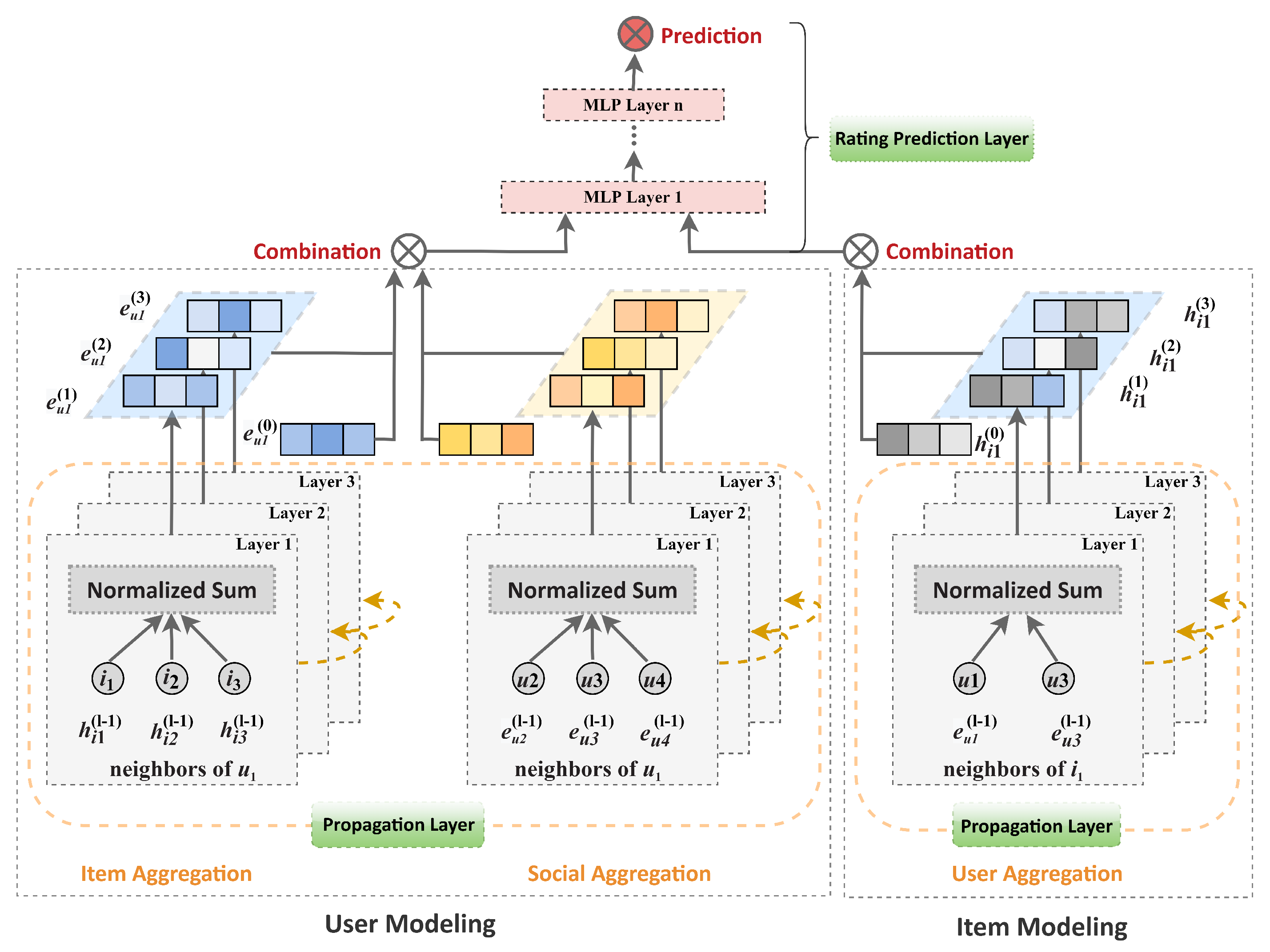
2. General design pipeline of GNNs
In this paper, we introduce models of GNNs in a designer view. We first present the general design pipeline for designing a GNN model in this section. Then we give details of each step such as selecting computational modules, considering graph type and scale, and designing loss function in Section 3 Instantiations of computational modules, 4 Variants considering graph type and scale, 5 Variants for different training settings, respectively. And finally, we use an example to illustrate the design process of GNN for a specific task in Section 6.
In later sections, we denote a graph as 𝐺=(𝑉,𝐸), where |𝑉|=𝑁 is the number of nodes in the graph and |𝐸|=𝑁𝑒 is the number of edges. 𝐴∈𝑅𝑁×𝑁 is the adjacency matrix. For graph representation learning, we use ℎ𝑣 and 𝑜𝑣 as the hidden state and output vector of node v. The detailed descriptions of the notations could be found in Table 1.
In this section, we present the general design pipeline of a GNN model for a specific task on a specific graph type. Generally, the pipeline contains four steps: (1) find graph structure, (2) specify graph type and scale, (3) design loss function and (4) build model using computational modules. We give general design principles and some background knowledge in this section. The design details of these steps are discussed in later sections.
2.1. Find graph structure
At first, we have to find out the graph structure in the application. There are usually two scenarios: structural scenarios and non-structural scenarios. In structural scenarios, the graph structure is explicit in the applications, such as applications on molecules, physical systems, knowledge graphs and so on. In non-structural scenarios, graphs are implicit so that we have to first build the graph from the task, such as building a fully-connected “word” graph for text or building a scene graph for an image. After we get the graph, the later design process attempts to find an optimal GNN model on this specific graph.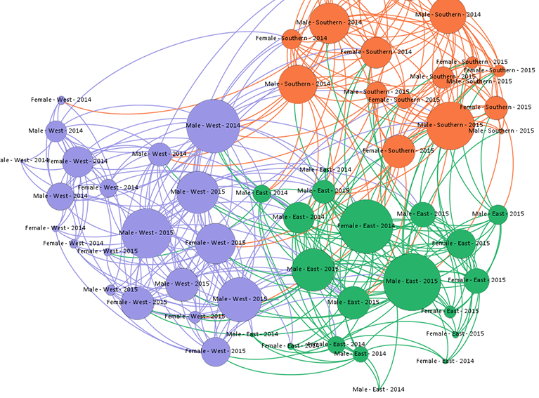
2.2. Specify graph type and scale
After we get the graph in the application, we then have to find out the graph type and its scale.
Graphs with complex types could provide more information on nodes and their connections. Graphs are usually categorized as:
- •
Directed/Undirected Graphs. Edges in directed graphs are all directed from one node to another, which provide more information than undirected graphs. Each edge in undirected graphs can also be regarded as two directed edges.
- •
Homogeneous/Heterogeneous Graphs. Nodes and edges in homogeneous graphs have same types, while nodes and edges have different types in heterogeneous graphs. Types for nodes and edges play important roles in heterogeneous graphs and should be further considered.
- •
Static/Dynamic Graphs. When input features or the topology of the graph vary with time, the graph is regarded as a dynamic graph. The time information should be carefully considered in dynamic graphs.
Note these categories are orthogonal, which means these types can be combined, e.g. one can deal with a dynamic directed heterogeneous graph. There are also several other graph types designed for different tasks such as hypergraphs and signed graphs. We will not enumerate all types here but the most important idea is to consider the additional information provided by these graphs. Once we specify the graph type, the additional information provided by these graph types should be further considered in the design process.
As for the graph scale, there is no clear classification criterion for “small” and “large” graphs. The criterion is still changing with the development of computation devices (e.g. the speed and memory of GPUs). In this paper, when the adjacency matrix or the graph Laplacian of a graph (the space complexity is 𝑂(𝑛2)) cannot be stored and processed by the device, then we regard the graph as a large-scale graph and then some sampling methods should be considered.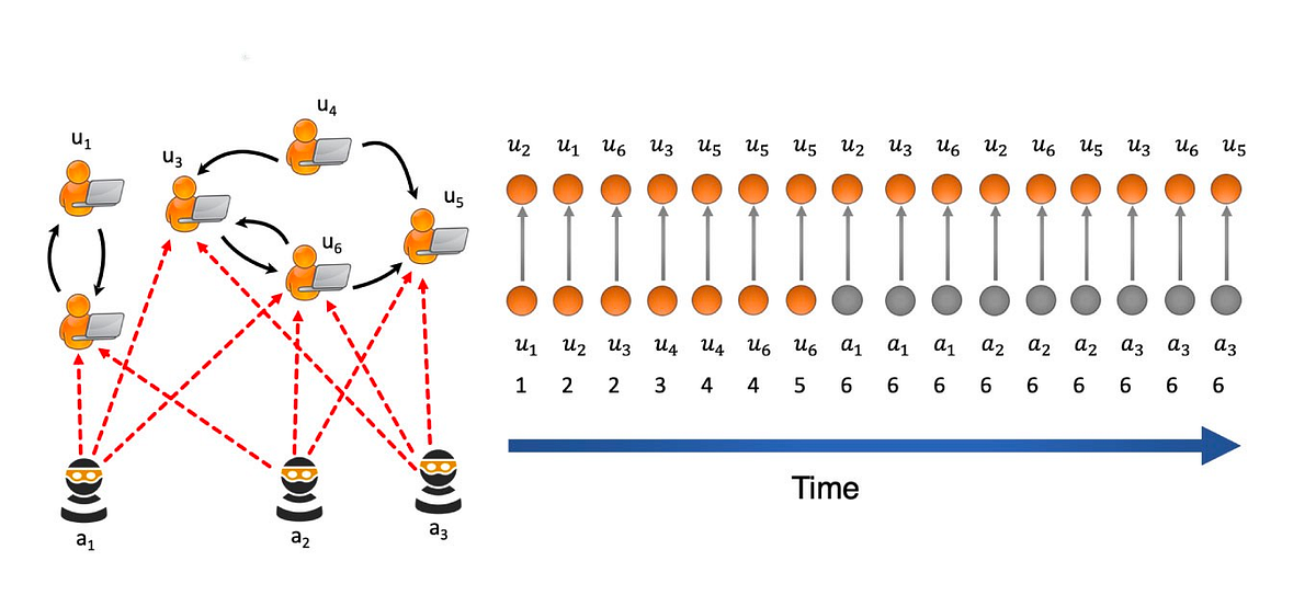
2.3. Design loss function
In this step we should design the loss function based on our task type and the training setting.
For graph learning tasks, there are usually three kinds of tasks:
- •
Node-level tasks focus on nodes, which include node classification, node regression, node clustering, etc. Node classification tries to categorize nodes into several classes, and node regression predicts a continuous value for each node. Node clustering aims to partition the nodes into several disjoint groups, where similar nodes should be in the same group.
- •
Edge-level tasks are edge classification and link prediction, which require the model to classify edge types or predict whether there is an edge existing between two given nodes.
- •
Graph-level tasks include graph classification, graph regression, and graph matching, all of which need the model to learn graph representations.
From the perspective of supervision, we can also categorize graph learning tasks into three different training settings:
- •
Supervised setting provides labeled data for training.
- •
Semi-supervised setting gives a small amount of labeled nodes and a large amount of unlabeled nodes for training. In the test phase, the transductive setting requires the model to predict the labels of the given unlabeled nodes, while the inductive setting provides new unlabeled nodes from the same distribution to infer. Most node and edge classification tasks are semi-supervised. Most recently, a mixed transductive-inductive scheme is undertaken by Wang and Leskovec (2020) and Rossi et al. (2018), craving a new path towards the mixed setting.
- •
Unsupervised setting only offers unlabeled data for the model to find patterns. Node clustering is a typical unsupervised learning task.
With the task type and the training setting, we can design a specific loss function for the task. For example, for a node-level semi-supervised classification task, the cross-entropy loss can be used for the labeled nodes in the training set.
2.4. Build model using computational modules
Finally, we can start building the model using the computational modules. Some commonly used computational modules are:
- •
Propagation Module. The propagation module is used to propagate information between nodes so that the aggregated information could capture both feature and topological information. In propagation modules, the convolution operator and recurrent operator are usually used to aggregate information from neighbors while the skip connection operation is used to gather information from historical representations of nodes and mitigate the over-smoothing problem.
- •
Sampling Module. When graphs are large, sampling modules are usually needed to conduct propagation on graphs. The sampling module is usually combined with the propagation module.
- •
Pooling Module. When we need the representations of high-level subgraphs or graphs, pooling modules are needed to extract information from nodes.
With these computation modules, a typical GNN model is usually built by combining them. A typical architecture of the GNN model is illustrated in the middle part of Fig. 2 where the convolutional operator, recurrent operator, sampling module and skip connection are used to propagate information in each layer and then the pooling module is added to extract high-level information. These layers are usually stacked to obtain better representations. Note this architecture can generalize most GNN models while there are also exceptions, for example, NDCN (Zang and Wang, 2020) combines ordinary differential equation systems (ODEs) and GNNs. It can be regarded as a continuous-time GNN model which integrates GNN layers over continuous time without propagating through a discrete number of layers.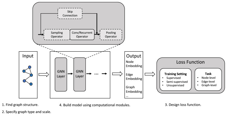
An illustration of the general design pipeline is shown in Fig. 2. In later sections, we first give the existing instantiations of computational modules in Section 3, then introduce existing variants which consider different graph types and scale in Section 4. Then we survey on variants designed for different training settings in Section 5. These sections correspond to details of step (4), step (2), and step (3) in the pipeline. And finally, we give a concrete design example in Section 6.
3. Instantiations of computational modules
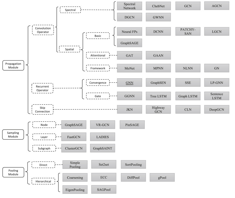
In this section we introduce existing instantiations of three computational modules: propagation modules, sampling modules and pooling modules. We introduce three sub-components of propagation modules: convolution operator, recurrent operator and skip connection in Section 3.1 Propagation modules – convolution operator, 3.2 Propagation modules – recurrent operator, 3.3 Propagation modules – skip connection respectively. Then we introduce sampling modules and pooling modules in Section 3.4 Sampling modules, 3.5 Pooling modules. An overview of computational modules is shown in Fig. 3.