Abstract
At the intersection of machine learning and quantum computing, quantum machine learning has the potential of accelerating data analysis, especially for quantum data, with applications for quantum materials, biochemistry and high-energy physics. Nevertheless, challenges remain regarding the trainability of quantum machine learning models. Here we review current methods and applications for quantum machine learning. We highlight differences between quantum and classical machine learning, with a focus on quantum neural networks and quantum deep learning. Finally, we discuss opportunities for quantum advantage with quantum machine learning.
Main
The recognition that the world is quantum mechanical has allowed researchers to embed well established, but classical, theories into the framework of quantum Hilbert spaces. Shannon’s information theory, which is the basis of communication technology, has been generalized to quantum Shannon theory (or quantum information theory), opening up the possibility that quantum effects could make information transmission more efficient1. The field of biology has been extended to quantum biology to allow for a deeper understanding of biological processes such as photosynthesis, smell and enzyme catalysis2. Turing’s theory of universal computation has been extended to universal quantum computation3, potentially leading to exponentially faster simulations of physical systems.
One of the most successful technologies of this century is machine learning (ML), which aims to classify, cluster and recognize patterns for large datasets. Learning theory has been simultaneously developed alongside of ML technology to understand and improve upon its success. Concepts such as support vector machines, neural networks and generative adversarial networks have impacted science and technology in profound ways. ML is now ingrained into society to such a degree that any fundamental improvement to ML leads to tremendous economic benefit.
Similarly to other classical theories, ML and learning theory can in fact be embedded into the quantum-mechanical formalism. Formally speaking, this embedding leads to the field known as quantum machine learning (QML)4,5,6, which aims to understand the ultimate limits of data analysis allowed by the laws of physics. Practically speaking, the advent of quantum computers, with the hope of achieving a so-called quantum advantage (as defined below) for data analysis, is what has made QML so exciting. Quantum computing exploits entanglement, superposition and interference to perform certain tasks with substantial speedups over classical computing, sometimes even exponentially faster. Indeed, while such speedup has already been observed for a contrived problem7, reaching it for data science is still uncertain even at the theoretical level, but this is one of the main goals for QML.
In practice, QML is a broad term that encompasses all of the tasks shown in Fig. 1. For example, ML can be applied to quantum applications such as discovering quantum algorithms8 or optimizing quantum experiments9,10, or a quantum neural network (QNN) can be used to process either classical or quantum information11. Even classical tasks can be viewed as QML when they are quantum inspired12. We note that the focus of this Perspective will be on QNNs, quantum deep learning and quantum kernels, even though the field of QML is quite broad and goes beyond these topics.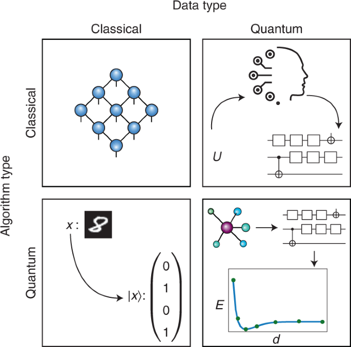
After the invention of the laser, it was called a solution in search of a problem. To some degree, the situation with QML is similar. The complete list of applications of QML is not fully known. Nevertheless, it is possible to speculate that all the areas shown in Fig. 2 will be impacted by QML. For example, QML will likely benefit chemistry, materials science, sensing and metrology, classical data analysis, quantum error correction and quantum algorithm design. Some of these applications produce data that are inherently quantum mechanical, and hence it is natural to apply QML (rather than classical ML) to them.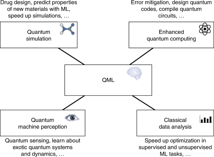
While there are similarities between classical and quantum ML, there are also some differences. Because QML employs quantum computers, noise from these computers can be a major issue. This includes hardware noise such as decoherence as well as statistical noise (that is, shot noise) that arises from measurements on quantum states. Both of these noise sources can complicate the QML training process. Moreover, nonlinear operations (for example, neural activation functions) that are natural in classical ML require more careful design of QML models due to the linearity of quantum transformations.
For the field of QML, the immediate goal for the near future is demonstrating quantum advantage, that is, outperforming classical methods, in a data science application. Achieving this goal will require keeping an open mind about which applications will benefit most from QML (for example, it may be an application that is inherently quantum mechanical). Understanding how QML methods scale to large problem sizes will also be required, including analysis of trainability (gradient scaling) and prediction error. The availability of high-quality quantum hardware13,14 will also be crucial.
Finally, we note that QML provides a new way of thinking about established fields, such as quantum information theory, quantum error correction and quantum foundations. Viewing such applications from a data science perspective will likely lead to new breakthroughs.
Framework
Data
As shown in Fig. 3, QML can be used to learn from either classical or quantum data, and thus we begin by contrasting these two types of data. Classical data are ultimately encoded in bits, each of which can be in a 0 or 1 state. This includes images, texts, graphs, medical records, stock prices, properties of molecules, outcomes from biological experiments and collision traces from high-energy physics experiments. Quantum data are encoded in quantum bits, called qubits, or higher-dimensional analogs. A qubit can be represented by the states |0〉, |1〉 or any normalized complex linear superposition of these two. Here, the states contain information obtained from some physical process such as quantum sensing15, quantum metrology16, quantum networks17, quantum control18 or even quantum analog–digital transduction19. Moreover, quantum data can also be the solution to problems obtained on a quantum computer: for example, the preparation of various Hamiltonians’ ground states.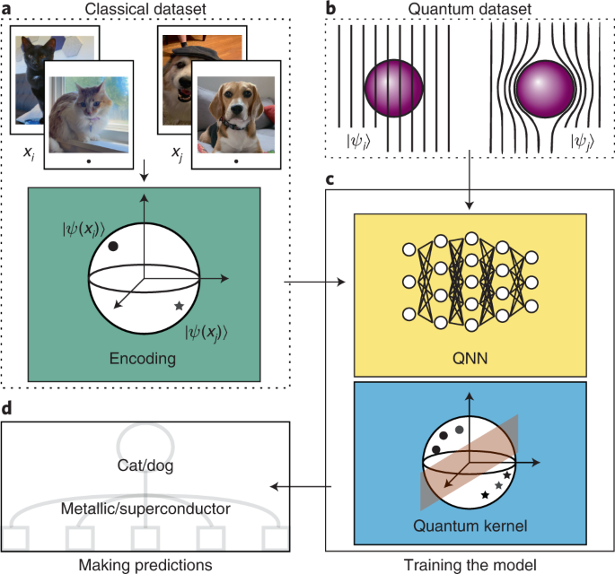
In principle, all classical data can be efficiently encoded in systems of qubits: a classical bitstring of length n can be easily encoded onto n qubits. However, the same cannot be said for the converse, since one cannot efficiently encode quantum data in bit systems; that is, the state of a general n-qubit system requires (2n − 1) complex numbers to be specified. Hence, systems of qubits (and more generally the quantum Hilbert space) constitute the ultimate data representation medium, as they can encode not only classical information but also quantum information obtained from physical processes.
In a QML setting, the term quantum data refers to data that are naturally already embedded in a Hilbert space 𝐻. When the data are quantum, they are already in the form of a set of quantum states {|ψj〉} or a set of unitaries {Uj} that could prepare these states on a quantum device (via the relation |ψj〉 = Uj|0〉). On the other hand, when the data x are classical, they first need to be encoded in a quantum system through some embedding mapping xj → |ψ(xj)〉, with |ψ(xj)〉 in 𝐻. In this case, the hope is that the QML model can solve the learning task by accessing the exponentially large dimension of the Hilbert space20,21,22,23.
One of the most important and reasonable conjectures to make is that the availability of quantum data will substantially increase in the near future. The mere fact that people will use the quantum computers that are available will logically lead to more quantum problems being solved and quantum simulations being performed. These computations will produce quantum datasets, and hence it is reasonable to expect the rapid rise of quantum data. Note that, in the near term, these quantum data will be stored on classical devices in the form of efficient descriptions of quantum circuits that prepare the datasets.
Finally, as our level of control over quantum technologies progresses, coherent transduction of quantum information from the physical world to digital quantum computing platforms may be achieved19. This would quantum mechanically mimic the main information acquisition mechanism for classical data from the physical world, this being analog–digital conversion. Moreover, we can expect that the eventual advent of practical quantum error correction24 and quantum memories25 will allow us to store quantum data on quantum computers themselves.
Models
Analyzing and learning from data requires a parameterized model, and many different models have been proposed for QML applications. Classical models such as neural networks and tensor networks (as shown in Fig. 1) are often useful for analyzing data from quantum experiments. However, due to their novelty, we will focus our discussion on quantum models using quantum algorithms, where one applies the learning methodology directly at the quantum level.
Similarly to classical ML, there exist several different QML paradigms: supervised learning (task based)26,27,28, unsupervised learning (data based)29,30 and reinforced learning (reward based)31,32. While each of these fields is exciting and thriving in itself, supervised learning has recently received considerable attention for its potential to achieve quantum advantage26,33, resilience to noise34 and good generalization properties35,36,37, which makes it a strong candidate for near-term applications. In what follows we discuss two popular QML models: QNNs and quantum kernels, shown in Fig. 3, with a particular emphasis on QNNs as these are the primary ingredient of several supervised, unsupervised and reinforced learning schemes.
Quantum neural networks
The most basic and key ingredient in QML models is parameterized quantum circuits (PQCs). These involve a sequence of unitary gates acting on the quantum data states |ψj〉, some of which have free parameters θ that will be trained to solve the problem at hand38. PQCs are conceptually analogous to neural networks, and indeed this analogy can be made precise: that is, classical neural networks can be formally embedded into PQCs39.
This has led researchers to refer to certain kinds of PQC as QNNs. In practice, the term QNN is used whenever a PQC is employed for a data science application, and hence we will use the term QNN in what follows. QNNs are employed in all three QML paradigms mentioned above. For instance, in a supervised classification task, the goal of the QNN is to map the states in different classes to distinguishable regions of the Hilbert space26. Moreover, in the unsupervised learning scenario of ref. 29, a clustering task is mapped onto a MAXCUT problem and solved by training a QNN to maximize distance between classes. Finally, in the reinforced learning task of ref. 32, a QNN can be used as the Q-function approximator, which can be used to determine the best action for a learning agent given its current state.
Figure 4 gives examples of three distinct QNN architectures where in each layer the number of qubits in the model is increased, preserved or decreased. In Fig. 4a we show a dissipative QNN40 which generalizes the classical feedforward network. Here, each node corresponds to a qubit, while lines connecting qubits are unitary operations. The term dissipative arises from the fact that qubits in a layer are discarded after the information forward-propagates to the (new) qubits in the next layer. Figure 4b shows a standard QNN where quantum data states are sent through a quantum circuit, at the end of which some or all of the qubits are measured. Here, no qubits are discarded or added as we go deeper into the QNN. Finally, Fig. 4c depicts a convolutional QNN11, where in each layer qubits are measured to reduce the dimension of the data while preserving its relevant features. Many other QNNs have been proposed41,42,43,44,45, and constructing QNN architectures is currently an active area of research.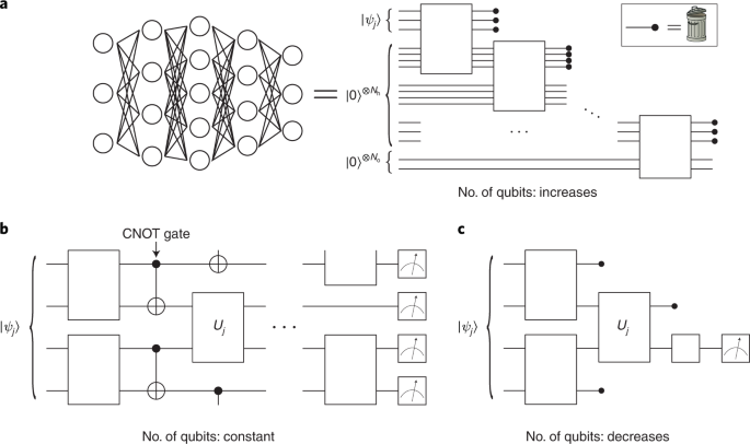
To further accommodate the limitation of near-term quantum computers, we can also employ a hybrid approach with models that have both classical and quantum neural networks46. Here, QNNs act coherently on quantum states while deep classical neural networks alleviate the need for higher-complexity quantum processing. Such hybridization distributes the representational capacity and computational complexity across both quantum and classical computers. Moreover, since quantum states generally have a mixture of classical correlations and quantum correlations, hybrid quantum–classical models allow for the use of quantum computers as an additive resource to increase the ability of classical models to represent quantum-correlated distributions. Applications of hybrid models include generating47 or learning and distilling information46 from multipartite-entangled distributions.
Quantum kernels
As an alternative to QNNs, researchers have proposed quantum versions of kernel methods26,28. A kernel method maps each input to a vector in a high-dimensional vector space, known as the reproducing kernel Hilbert space. Then, a kernel method learns a linear function in the reproducing kernel Hilbert space. The dimension of the reproducing kernel Hilbert space could be infinite, which enables the kernel method to be very powerful in terms of expressiveness. To learn a linear function in a potentially infinite-dimensional space, the kernel trick48 is employed, which only requires efficient computation of the inner product between these high-dimensional vectors. The inner product is also known as the kernel48. Quantum kernel methods consider the computation of kernel functions using quantum computers. There are many possible implementations. For example, refs. 26,28 considered a reproducing kernel Hilbert space equal to the quantum state space, which is finite dimensional. Another approach13 is to study an infinite-dimensional reproducing kernel Hilbert space that is equivalent to transforming a classical vector using a quantum computer. It then maps the transformed classical vectors to infinite-dimensional vectors.
Inductive bias
For both QNNs and quantum kernels, an important design criterion is their inductive bias. This bias refers to the fact that any model represents only a subset of functions and is naturally biased towards certain types of function (that is, functions relating the input features to the output prediction). One aspect of achieving quantum advantage with QML is to aim for QML models with an inductive bias that is inefficient to simulate with a classical model. Indeed, it was recently shown49 that quantum kernels with this property can be constructed, albeit with some subtleties regarding their trainability.
Generally speaking, inductive bias encompasses any assumptions made in the design of the model or the optimization method that bias the search of the potential models to a subset in the set of all possible models. In the language of Bayesian probabilistic theory, we usually call these assumptions our prior. Having a certain parameterization of potential models, such as QNNs, or choosing a particular embedding for quantum kernel methods13,14,26 is itself a restriction of the search space, and hence a prior. Adding a regularization term to the optimizer or modulating the learning rate to keep searches geometrically local also adds inherently a prior and focuses the search, and thus provides inductive bias.
Ultimately, inductive biases from the design of the ML model, combined with a choice of training process, are what make or break an ML model. The main advantage of QML will then be to have the ability to sample from and learn models that are (at least partially) natively quantum mechanical. As such, they have inductive biases that classical models do not have. This discussion assumes that the dataset to be represented is quantum mechanical in nature, and is one of the reasons why researchers typically believe that QML has greater promise for quantum rather than classical data.
Training and generalization
The ultimate goal of ML (classical or quantum) is to train a model to solve a given task. Thus, understanding the training process of QML models is fundamental for their success.
Consider the training process, whereby we aim to find the set of parameters θ that lead to the best performance. The latter can be accomplished, for instance, by minimizing a loss function θ𝐿(θ) encoding the task at hand. Some methods for training QML models are leveraged from classical ML, such as stochastic gradient descent. However, shot noise, hardware noise and unique landscape features often make off-the-shelf classical optimization methods perform poorly for QML training. (This is due to the fact that extracting information from a quantum state requires computing the expectation values of some observable, which in practice need to be estimated via measurements on a noisy quantum computer. Hence, given a finite number of shots (measurement repetitions), these can only be resolved up to some additive errors. Moreover, such expectation values will be subject to corruption due to hardware noise.) This realization led to development of quantum-aware optimizers, which account for the quantum idiosyncrasies of the QML training process. For example, shot-frugal optimizers50,51,52,53 can employ stochastic gradient descent while adapting the number of shots (or measurements) needed at each iteration, so as not to waste too many shots during the optimization. Quantum natural gradient54,55 adjusts the step size according to the local geometry of the landscape (on the basis of the quantum Fisher information metric). These and other quantum-aware optimizers often outperform standard classical optimization methods in QML training tasks.
For the case of supervised learning, we are interested not only in learning from a training dataset but also in making accurate predictions on (generalizing to) previously unseen data. This translates into achieving small training and prediction errors, with the second usually hinging on the first. Thus, let us now consider prediction error, also known as generalization error, which has been studied only very recently for QML13,14,35,37,56,57. Formally speaking, this error measures the extent to which a trained QML model performs well on unseen data. Prediction error depends on the training error as well as the complexity of the trained model. If the training error is large, the prediction error is also typically large. If the training error is small but the complexity of the trained model is large, then the prediction error is likely still large. The prediction error is small only if training error is itself small and the complexity of the trained model is moderate (that is, sufficiently smaller than training data size)14,35. The notion of complexity depends on the QML model. We have a good understanding of the complexity of quantum kernel methods13,14, while more research is needed on QNN complexity. Recent theoretical analysis of QNNs shows that their prediction performance is closely linked to the number of independent parameters in the QNN, with good generalization obtained when the number of training data is roughly equal to the number of parameters35. This gives the exciting prospect of using only a small number of training data to obtain good generalization.

